nilsschneider.de

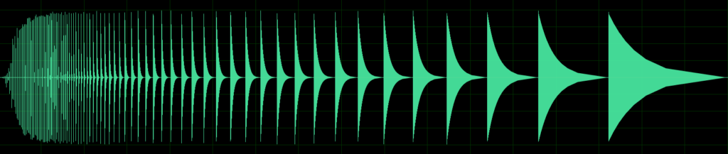
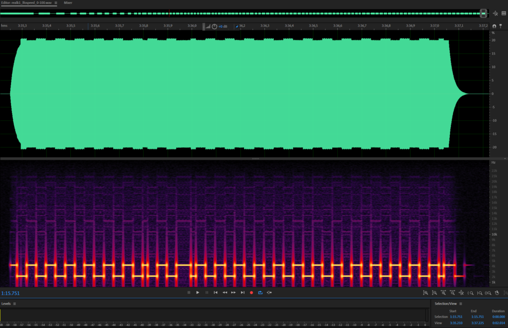
The K1 is full of aliasing, which is obvious when taking a look at the waveform recordings (see previous article).

Nowadays, it would be pretty straightforward to eliminate the aliasing by doing bandlimited interpolation of the waveforms. But…

What we have to be aware of is that a lot of singles actively make use of aliasing to produce their unique sound. So instead of preventing aliasing, the goal is to recreate the aliasing behavior of the original K1.

What is Aliasing?

To do that, firstly, we have to know what happens when aliasing occurs. Every digital audio device works at a specific sampling rate. For example, a CD player works at a sampling rate of 44100 Hz, or 44,1 KHz. The nyquist theorem states that, given a sampling rate of n, a maximum frequency of n/2 can be represented in an audio stream. In the CD player example, the maximum frequency that can be stored on a CD is 22050 Hz.

If a frequency is generated at runtime, special care needs to be taken to ensure that every frequency is always less than half the sampling rate, aka the nyquist frequency. If the frequency is too high, it starts to mirror at the nyquist frequency, giving unexpected results.

An example: If your audio interface runs at a frequency of 44100 Hz but you try to generate a sine wave of 30000 Hz, it is mirrored at 22050 Hz and begins to fall downwards. Lets do the math:
30000 Hz – 22050 Hz =7950 Hz, so the desired frequency is 7950 Hz too high to be represented correctly.
Mirrored at the nyquist frequency: 22050 Hz – 7950 Hz = 14100 Hz.

So, although we wanted to play a sine wave at 30000 Hz, what we get to hear is a sine wave at 14100 Hz and this is what we call aliasing.

Aliasing on the K1

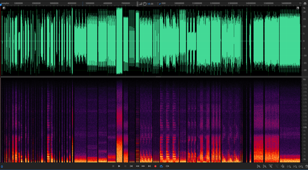
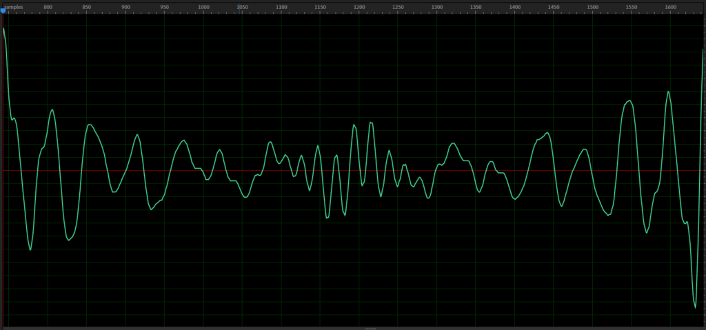
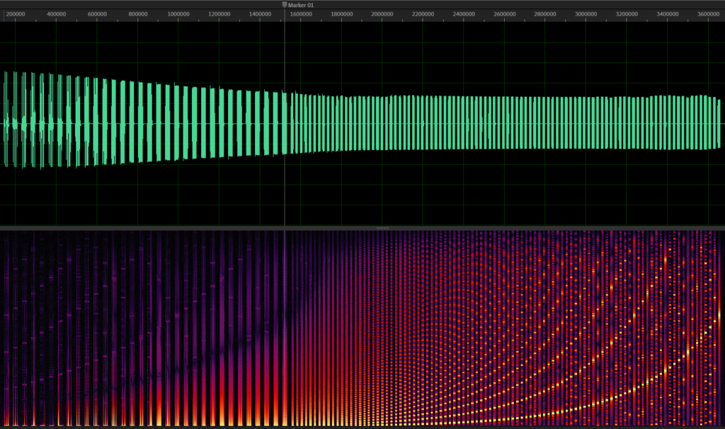
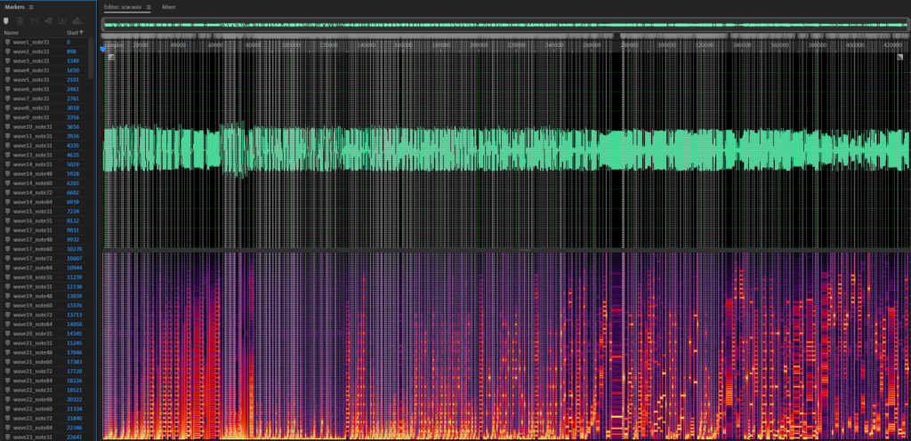
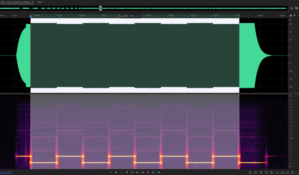
To see aliasing on the K1, take a look at this image:

This is one of the waveform recordings where I played every note from 0 to 127. It starts to alias, but at a frequency that is not known yet.

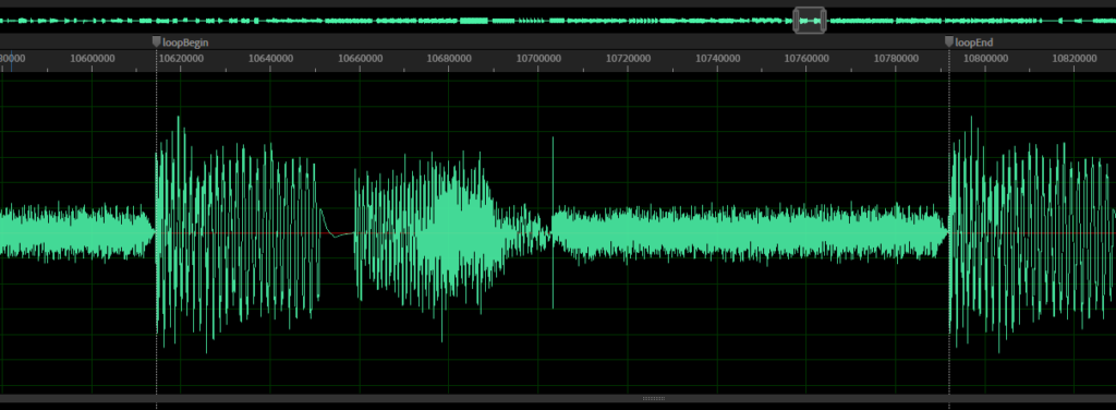
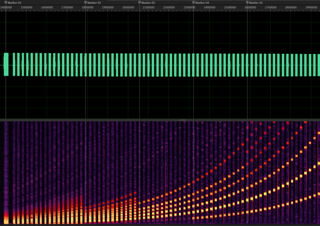
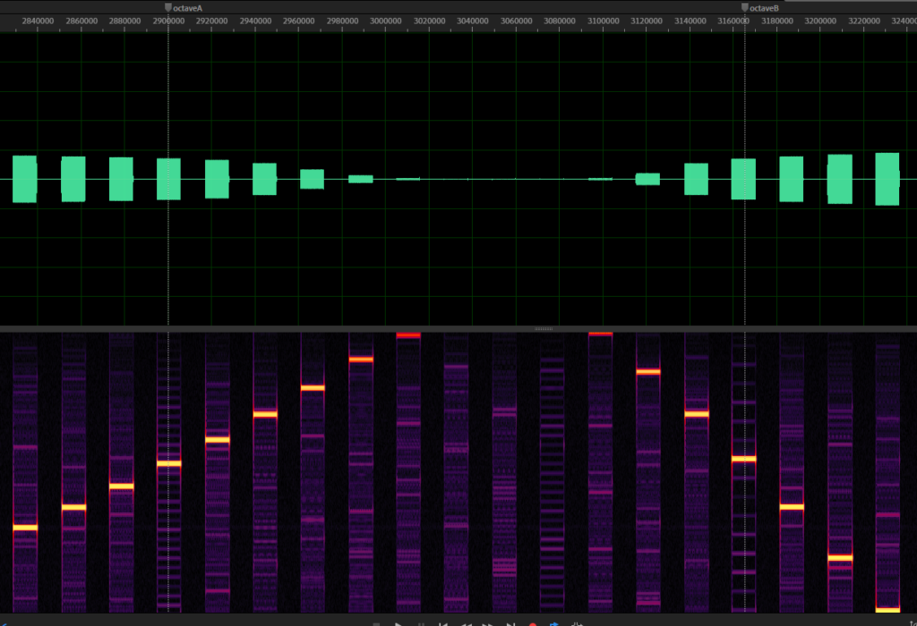
If you look closer, I added two markers here. The first one is an arbitrary note, the second one is 12 notes away from the first one. I did this because that is exactly one octave higher (note: frequency doubles with each octave) so we can expect that the frequency should be twice as high as the first one, but this is not the case, obviously.

At the first marker, we have a sine wave of roughly 16630 Hz. This should result in the second sine wave being at 33260 Hz. But at the second marker, we observe a sine wave with the frequency of about 16820 Hz instead.

Having both of these values, we can calculate the frequency at which the second sine is mirrored: 33260 Hz – 16820 Hz = 16440 Hz. Half of this value is 8220 Hz and if we add this to the frequency of the first marker the result is 25040 Hz.

The result is our nyquist frequency, which is equal to half sampling rate. If we double this value we get 50080 Hz.

As the FFT frequency analysis is never completely precise and I expect that Kawai has chosen some easy to remember value, I rounded the result which gives us a sampling rate for the K1 of 50000 Hz

Knowing that the sampling rate of the K1 is 50 KHz, I adjusted my emulation to run at the same sampling rate. Furthermore, the waveform playback interpolation has to be kept very basic, for now I have chosen to use very simple linear interpolation. The result is aliasing, identical to the original K1.

A single that makes use of the aliasing is, again, IA-5 Visitors. I added the single to the audio examples, feel free to listen to it here.

Just in case you wonder if that limits the VSTi plugin in any way, don’t worry. It will work on any host sampling rate, I added high quality band limited resampling code that is based on CCRMA/Stanford, as written here: https://ccrma.stanford.edu/~jos/resample/

The K1 emulation engine will always run at 50 KHz and the result will be converted to match the sampling rate of the host.

While the waveform pack by Chvad was pretty good to have something to start with, I had some issues, both for the PCM based waveforms and the single cycle waveforms.

PCM waveforms

Chvad sampled the waveforms at note number D4, which sounds good when being played back in a wave player, but the problem it causes is that you lose a lot of the high frequency spectrum when being played on lower midi notes.
Secondly, there is no chance to filter any noise that is emitted by the K1.

Therefore, I decided to sample the PCM waveforms on note D1 instead.

Recording was pretty straightforward, I played the same midi note over and over again and selected the different waveforms inbetween my note pressed. The result looked like this:

To make my life a little easier, I wrote a tool to help extracting single files out of this big recording.
What the tool does is, firstly, it detects blocks of silence and audible data. What I use this for is to know when a new waveform starts. This gives a total amount of 52 blocks of audio data, with silence in between them, which matches the PCM waveforms 205-256.
Secondly, as there are waveforms that need to be looped during playback, I created code to detect them. My tool can read wave markers and work on loops according to these markers. There are two types of loops that I need to support:

• Loops that I define manually with a specified start and end point
• Loops where I only define a region where a loop is, together with a maximum length. The loop start and end is then detected automatically

After I had defined all required markers, the whole file looked like this:

After executing my tool, the output was a nice list of loopable PCM waveforms that were ready to be used in my K1 emulation VSTi

Single Cycle Waveforms

What always made me wondering is the fact that the single Visitors appears to have some sine wave sound, whose pitch is modified by the LFO, but when inspecting how the single is made, you’ll notice that there is no sine wave selected as a source at all. The waveform that is driven by the LFO is wave 204, which sounds quite different and looks like this:

It is not a sine wave at all, it sounds more like some synthesized waveform, frankly, the K1 manual names this waveform SYNTH_01

While testing something else on the real K1, I noticed something strange. I pressed a note and modified the coarse tune while holding the note down. When I released the note and retriggered it, the sound was different! I tested this a couple of times and every time, the sound was different after retriggering when I modified the coarse tune while holding a note.

I had an idea what that means and after doing a test recording of a waveform for all notes, ranging from 0 to 127 I had the proof: Single cycle waveforms are multisamples!

If you take a closer look at the image, especially at the frequency spectrum in the lower part, you’ll see that some harmonics get lost as the note number is rising.

That explained a lot. No wonder that I never had that original K1 sound. As the recordings by Chvad were only one version of each waveform, I had to record every single cycle waveform again, but this time for each note number.

It took a lot of hours to get this done but it was definitely worth it. I’ve setup a simple track in Cubase to play all notes from 0 to 127 and recorded all 204 single cycle waveforms.
It turned out that not every waveform contains multisamples. And for some of them, the way they use them is really strange. Usually, if you do this, you cut harmonics before they reach the nyquist frequency to prevent aliasing. But in the case of the K1, this is not (properly) done. Some multisamples clearly change the tone when you play on the keyboard, for others, they even make it worse by adding harmonics instead of removing them, which increases the aliasing even more.
Some examples:

As you can see, there are a lot of variantions. If you want an exact recreation, you need to take all different multisamples into account.

Single Cycle Waveforms conversion tool

Once more, I extended my tool to deal with these recordings. I manually added markers to the notes that I want to extract. You can see the markers in the screenshots above. My tool uses these markers to extract loops of the waveforms at their respective positions and exports to single files.

Notice the note numbers on the left. The tool names these markers to make sure that the root note of the loop is known, so the playback is done at the correct pitch.

After all 204 files are created, they are merged into a single file, which allows me to load them more easily. The result is a 1,66 MB wave file with over 500 markers in total, named as wave120_note84, etc.

The sound has improved a lot, in many areas, its very similar to a K1 now, just as it should.
What I didn’t do yet, as it is a lot of manual work, is to clean up the recordings a bit. There is a bit of K1 noise that could be easily filtered out, but it would need to be a manual process for each waveform and for each multisample, as the used frequencies are different for each one, leading to over 500 manual tweaks.

Another minor thing is that, although the original K1 wave rom consisted only of 512kb of data, my data size is about 24mb in total as I have every waveform as 32 bits floating point data. It is not much nowadays for a plugin to be that large, but an optimization would be nice.

Update: New Audio Demo is here

Recently, I worked in lots of different areas. I re-recorded all wavetables (separate article will follow), reworked the envelope timings, implemented velocity curves, measured LFO speeds and more.

I thought its about time for some audio demos. I recorded this using the current state of the VST plugin. Of course, there are still a lot of issues, but a lot of presets are running fine already.

In the audio demo above, you hear the following factory presets (in order of appearance):

• iA-5 Return Home
• IB-3 Jazz Harp
• IA-5 Visitors
• IA-3 String Pad
• IC-7 Terminator

The only thing I added is a bit of reverb and EQ. Let me know what you think!

Next step for me was to analyze the envelope values and velocity mappings. Because the LFO speed analysis was quite cumbersome, I decided to create a tool to analyse further parameters to make it a little easier for me.

For the envelope decay & release, I noticed that several singles share the same setting for both values. This is mostly used for drum presets but for some others, too. I verified it on the K1m and confirmed that this was the case.

Then, I used my simple init preset again and recorded note presses while adjusting the envelope decay value from 0 to 100. The result was this very long recording:

The largest envelope decay/release time is 2:44 minutes! But that was not the only thing I observed, I also noticed that the envelope decay is not purely logarithmic, but is a mixture of some logarithmic key points with linear interpolation between them. For longer release times, this is pretty obvious when looking at the waveform, but luckily not very noticeable when listening to it.

Having the recording ready, I created a little wave analyzer whose purpose is to dump envelope durations. It analyzes the waveform to find where a note begins and tracks the duration until the wave falls below an adjustable threshold and logs the time.
While this doesn’t work properly for the very short attack times (I measured them manually instead), it saved a lot of time.

Unfotunately, I had no chance to analyze the envelope attack times, as my K1m is broken here, but I assumed that they are identical and first tests confirm that, so I have all of three (Attack, Decay, Release) finished by now.

I extended this little tool to output gain values. I used it for the various velocity curves, envelope levels, sustain levels and so on.

As you can see in the picture above, the velocity curve is a little bit steppy. Apparently the resolution is not very good. Anyway, I used the same low resolution in my emulator to closely match the original device.

Meanwhile, I’ve got a real Kawai K1m to analyze the machine. Unfortunately, it has got a little defect: The envelope attack is broken. With values above 50, the sound gets quiter and quieterand if you raise the attack above values of 68, there is no sound anymore.
I ordered an Eprom to upgrade the firmware from version 1.1 to version 1.5, but unfortunately this didn’t have any effect, the problem persists. I checked the soldering points, but I have not been able to find anything obvious. I contacted Kawai, maybe they can help to identify the problem.

Nevertheless, there is plenty of stuff I can do to analyze the device, even though the attack is not working properly (yet!).

I started to analyze the LFO speeds. I wanted to know which LFO speed value, ranging from 0 to 100, results in what length of one LFO loop in seconds. To do that, I created a very simple patch where the LFO is of type square and modulates the frequency of a sine. Then, I started recording and stepped through all values from 0 to 100 and pressed a note on my keyboard for each value.

The result looks like this:

After having done that, a lot of cumbersome work had to be done. I had to select an LFO loop in the wave editor and write down its length. For the higher LFO frequencies, I selected multiple loops (up to 16) and divided by 16 afterwards to get the correct average value as it turned out that the LFO precision is very low on the K1.
A picture of the highest LFO speed can be seen below. You can notice how the frequency is not constant, but jumps a lot.

After having entered everything in a Google Spreadsheet, I created a diagram to check for errors and tweaked the values manually here or there to get rid of precision issues.

Afterwards, I added the final result to my emulator which now has proper LFO speed values by using a table lookup for all possible values from 0-100.

It was a lot of work, but was completely worth it. I did several A-B checks against the real K1m that I now have and the LFO speeds are completely identical, just as it should be!